3D FV Navier Stokes Example

In the scope of computational fluid dynamics (CFD), the Navier Stokes (NS) equations are of great importance as they can be used to model the behavior of fluids or fluid-like substances, assuming knowledge of its initial state and boundary conditions. Typical applications are the water flow in a pipe, ocean currents or even the air flow around a car or wing. In this tutorial, we take a look at the incompressible NS equations which describe the dynamic flow of incompressible fluid, with the unknowns being the pressure and velocity as functions of space and time variables. In this example, we only cover Newtonian fluids.

Note that this tutorial covers more advanced topics than others. Hence, it is strongly recommended to follow the reading order which can be found here. For the sake of compactness, only the most relevant parts of the implementation are covered. However, the complete program specification can be found in the files listed in the code generation chapter.

Introduction

In this tutorial, we discretize the NS equation using the Finite Volumes (FV) method. Here, we use a non-linear Multigrid method, also known as Full Approximation Scheme (FAS).

Finite Volumes

While it would be also possible to discretize the NS equations using Finite Differences (FD), this example’s focus lies on a FV discretization. In contrast to FD, one does not discretize the operators but considers the whole equation at once. Moreover, the grid data is located at the cell centers where data is assumed to be equal across one cell.

Independent from the NS equations, we first consider the following 2D problem to introduce the FV method:

\[\frac{\delta}{\delta x} u + \frac{\delta}{\delta y} u = \nabla \cdot u = f\]

Here, \(u\) is the unknown and \(f\) the right-hand side. After integrating over the whole physical domain, we get the following:

\[\iint_{\Omega} \nabla \cdot u \: dx dy = \iint_{\Omega} f \: dx dy\]

By splitting the physical domain into multiple cells, we can now solve the equation for the computational domain, i.e. by solving the integral for each cell, which will be also denoted as control volumes \(\Omega_{i,j} \in \Omega\).

\[\iint_{\Omega_{i,j}} \nabla \cdot u \: dx dy = \iint_{\Omega} f \: dx dy\]

By applying the divergence theorem, the integral on the left-hand side is now replaced by a surface integral

\[\oint_{\delta \Omega_{i,j}} u \cdot \hat{\mathbf{n}} \: dx dy\]

with \(\hat{\mathbf{n}}\) being the surface normal. For axis-aligned uniform grids with step sizes \(\Delta x\) and \(\Delta y\), this can be simplified to:

\[\Delta y \: u_{i+1/2,j} - \Delta y \: u_{i-1/2, j} + \Delta x \: u_{i, j+1/2} - \Delta x \: u_{i, j-1/2} = \Delta x \Delta y \: f_{i,j}\]

with half indices indicating an evaluation of quantities at the cell interfaces. There are multiple approaches to compute the values at the interfaces. The most simple one is merely building the mean value of two neighboring cells.

For second order derivatives, for instance the Poisson’s equation \(-\Delta u = - \nabla^2 u = f\), the integration over the control volumes looks as follows:

\[-\iint_{\Omega_{i,j}} \nabla^2 u \: dx dy = \iint_{\Omega_{i,j}} f \: dx dy\]

After applying Green’s identities, this is simplified to:

\[-\oint_{\delta \Omega_{i,j}} \nabla u \cdot \hat{\mathbf{n}} \: dx dy = \iint_{\Omega_{i,j}} f \: dx dy\]

So, instead of evaluating the quantities at the cell interfaces we evaluate their derivatives. These can be obtained using the FD method. For an axis-aligned uniform grid, we get:

\[-\Delta y \frac{u_{i+1, j} - u_{i,j}}{\Delta x} + \Delta y \frac{u_{i, j} - u_{i-1,j}}{\Delta x} -\Delta x \frac{u_{i, j+1} - u_{i,j}}{\Delta y} + \Delta x \frac{u_{i, j} - u_{i,j-1}}{\Delta y} = \Delta x \Delta y \: f_{i,j}\]

Problem Description

With the theoretical background in the FV method in mind we can begin discretizing the incompressible Navier-Stokes equations. At first we take a look at the continuous formulation of the problem on domain \(\Omega \in [0, \frac{1}{10}]^3\):

\[ \begin{align}\begin{aligned}\rho \Big( \frac{\delta \mathbf{u}}{\delta t} + (\mathbf{u} \cdot \nabla) \mathbf{u} \Big) - \mu \nabla^2 \mathbf{u} + \nabla p = \tilde{\mathbf{f}}\\\nabla \cdot \mathbf{u} = 0\end{aligned}\end{align} \]

With \(\mathbf{u}\) being the unknown and \(p\) the pressure. Moreover, \(\rho\) denotes the density and \(\mu\) the dynamic viscosity. The second equation is known as the continuity equation. For the kinematic viscosity \(\nu = \frac{\mu}{\rho}\) one can reformulate the upper equation by dividing by \(\rho\):

\[ \begin{align}\begin{aligned}\frac{\delta \mathbf{u}}{\delta t} + (\mathbf{u} \cdot \nabla) \mathbf{u} - \nu \nabla^2 \mathbf{u} + \frac{1}{\rho} \nabla p = \mathbf{f}\\\nabla \cdot \mathbf{u} = 0\end{aligned}\end{align} \]

Here, our right-hand side is the gravity \(\mathbf{g}\). Reformulated as scalar equations, this yields:

\[ \begin{align}\begin{aligned}\frac{\delta u}{\delta t} + u \frac{\delta u}{\delta x} + v \frac{\delta u}{\delta y} + w \frac{\delta u}{\delta z} - \nu \Big( \frac{\delta^2 u}{\delta x^2} + \frac{\delta^2 u}{\delta y^2} + \frac{\delta^2 u}{\delta z^2} \Big) + \frac{1}{\rho} \frac{\delta p}{\delta x} = f_u\\\frac{\delta v}{\delta t} + u \frac{\delta v}{\delta x} + v \frac{\delta v}{\delta y} + w \frac{\delta v}{\delta z} - \nu \Big( \frac{\delta^2 v}{\delta x^2} + \frac{\delta^2 v}{\delta y^2} + \frac{\delta^2 v}{\delta z^2} \Big) + \frac{1}{\rho} \frac{\delta p}{\delta y} = f_v\\\frac{\delta w}{\delta t} + u \frac{\delta w}{\delta x} + v \frac{\delta w}{\delta y} + w \frac{\delta w}{\delta z} - \nu \Big( \frac{\delta^2 w}{\delta x^2} + \frac{\delta^2 w}{\delta y^2} + \frac{\delta^2 w}{\delta z^2} \Big) + \frac{1}{\rho} \frac{\delta p}{\delta z} = f_w\\ \frac{\delta}{\delta x} u +\frac{\delta}{\delta y} v + \frac{\delta}{\delta z} w = 0\end{aligned}\end{align} \]

Staggered Grids

Locating all quantities, e.g. the velocity and pressure, on the same grid location can lead to stability issues. One prominent example is the odd-even decoupling of pressure and velocity which may lead to checkerboard patterns in the solutions. Therefore, as a countermeasure we employ so-called staggered grids. A 2D example is depicted below. On the left side, the different variable localizations are shown and on the right side, staggered control volumes are depicted.

Fig. 1: 2D staggered grid.

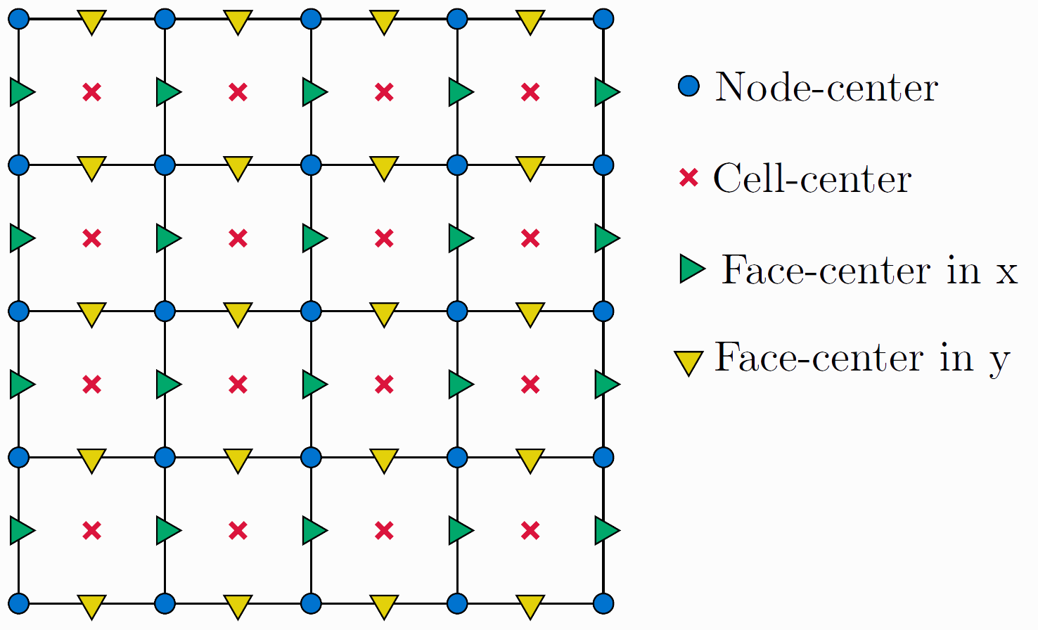
Note that besides regular node- or cell-centered quantities we now also have face-centered ones. These are effectively used to implement staggered grids. Face-centered variables have a face dimension which equals the stagger dimension, i.e. the dimension in which cell-centered variables need to be shifted to concur with the cell interfaces. In ExaStencils, this is implemented such that in all dimensions except the stagger dimension the variables are treated as cell-centered. In the stagger dimension they are treated as node-centered.

Integrate Functions

As already mentioned, we use the FV method to discretize our continuous terms. Since integrations are ubiquitous in FV discretizations, e.g. for the integration over a specific boundary of a (potentially staggered) control volume, ExaStencils provides special constructs for these operations, namely integrate functions. Examples for them are shown below:

Integrate Functions in ExaSlang

// integrate over interfaces of regular grid cells
integrateOverEastFace ( expr )

// integrate over interfaces of y-staggered cells
integrateOverYStaggeredWestFace ( u )

// integrate function call with offset
integrateOverSouthFace@[0, 1] ( p )

Their function name always begins with integrateOver followed by an optional stagger dimension (XStaggered, YStaggered or ZStaggered) and a target interface (EastFace, NorthFace, TopFace, …). Moreover, these functions not only take constants, variables or field accesses as argument, but also allow more complex expressions to be passed. Additionally, as shown in line 8 of the above code snippet, offsets for the function call can be specified.

Discretization

For a better overview, this section has been split into the discretization of the two equations, namely the NS and the continuity equation.

\[ \begin{align}\begin{aligned}\iiint_{\Omega} \frac{\delta \mathbf{u}}{\delta t} + (\mathbf{u} \cdot \nabla) \mathbf{u} - \nu \nabla^2 \mathbf{u} + \frac{1}{\rho} \nabla p \: dx dy dz = \iiint_{\Omega} \mathbf{f} \: dx dy dz\\\iiint_\Omega \nabla \cdot \mathbf{u} \: dx dy dz = 0\end{aligned}\end{align} \]

We begin with the continuity equation since the necessary steps are rather simple. Here, we again apply the divergence theorem and integrate over the non-staggered control volume \(\Omega_{i,j,k}\):

\[\oint_{\delta \Omega_{i,j,k}} \mathbf{u} \cdot \hat{\mathbf{n}} \: dx dy dz = 0\]

The discretization of the NS equation is more complex. Thus, we first break the left-hand side of the equation down into four parts:

1. The time derivative: \(\displaystyle{ \frac{\delta \mathbf{u}}{\delta t} }\).

2. The non-linear convective term: \(\displaystyle{ \Big( \mathbf{u} \cdot \nabla \Big) \mathbf{u} }\).

3. The diffusive term: \(\displaystyle{ \nu \nabla^2 \mathbf{u} }\).

4. The pressure coupling: \(\displaystyle{ \frac{1}{\rho} \nabla p }\).

In the following, the discretization of each part will be viewed separately and will be plugged together in the end again.

Time Derivative

We first discretize the first-order time derivative:

\[\iiint_{\Omega} \frac{\delta \mathbf{u}}{\delta t} \: dx dy dz = \frac{\delta \mathbf{u}}{\delta t} \iiint_{\Omega} 1 \: dx dy dz\]

For the approximation of the time derivative, we use a straightforward backwards difference, i.e.

\[\frac{\delta \mathbf{u}^{n+1}}{\delta t} \approx \frac{\mathbf{u}^{n+1} - \mathbf{u}^n}{\Delta t}\]

where \(n\) denotes the current time step and \(\Delta t\) the time step size.

Diffusion

For the diffusion, we simply apply Green’s identities again:

\[- \iiint_{\Omega} \nu \nabla^2 \mathbf{u} \: dx dy dz = -\oint_{\delta \Omega} \nu \nabla \mathbf{u} \cdot \hat{\mathbf{n}} \: dx dy dz\]

Formulated as integrals over the control volumes and split up into scalar equations, this yields:

\[ \begin{align}\begin{aligned}-\oint_{\delta \Omega_{i + 1/2, j, k}} \frac{\delta}{\delta x} u \cdot \hat{\mathbf{n}} \: dx dy dz\\-\oint_{\delta \Omega_{i, j + 1/2, k}} \frac{\delta}{\delta y} v \cdot \hat{\mathbf{n}} \: dx dy dz\\-\oint_{\delta \Omega_{i, j, k + 1/2}} \frac{\delta}{\delta z} w \cdot \hat{\mathbf{n}} \: dx dy dz\end{aligned}\end{align} \]

with \(\Omega_{i,j,k}\) being the non-staggered volume for the cell \((i, j, k)\) and \(\Omega_{i + 1/2, j, k}\), \(\Omega_{i, j + 1/2, k}\) and \(\Omega_{i, j, k + 1/2}\) being the staggered control volumes in x-, y- and z-direction. As mentioned in the FV chapter, we evaluate the derivatives using FD.

Convection

Afterwards, we inspect the non-linear convective term and simplify it:

\[\iiint_\Omega (\mathbf{u} \cdot \nabla) \mathbf{u} \: dx dy dz = \oint_{\delta \Omega} \mathbf{u} ( \mathbf{u} \cdot \hat{\mathbf{n}} ) \: dx dy dz\]

And rewritten as scalar equations:

\[ \begin{align}\begin{aligned}\oint_{\delta \Omega_{i + 1/2, j, k}} u ( \mathbf{u} \cdot \hat{\mathbf{n}} ) \: dx dy dz\\\oint_{\delta \Omega_{i, j + 1/2, k}} v ( \mathbf{u} \cdot \hat{\mathbf{n}} ) \: dx dy dz\\\oint_{\delta \Omega_{i, j, k + 1/2}} w ( \mathbf{u} \cdot \hat{\mathbf{n}} ) \: dx dy dz\end{aligned}\end{align} \]

Since some algorithmic components, e.g. a (linear) smoother in the solver, require a linearized version of these non-linear terms, linearization techniques must be applied. In this tutorial the focus will lie on the Picard linearization, also known as frozen or lagged coefficients. Generally, the linearization can be done locally, i.e. for a single cell or a small set of cells, or globally, i.e. for the whole system of equations. This tutorial is structured such that the local variant is the focal point, but some remarks to the global variant can be found in the global linearization excursion.

As the name frozen coefficients implies, the gist is to freeze parts of the non-linear term. For the convective term this yields:

\[(\mathbf{u}^{k+1} \cdot \nabla) \mathbf{u}^{k+1} \approx (\mathbf{u}^{k} \cdot \nabla) \mathbf{u}^{k+1}\]

Here, the frozen parts are marked with the superscript \(k\), whereas the remaining parts are denoted by \(k + 1\). In contrast to the frozen parts, the remaining ones can be solved or updated for.

In order to provide this knowledge to the code generator, ExaStencils introduced so-called frozen field access. For instance, a frozen access to the \(\mathbf{u}\) vector’s y-component \(v\) would look like this:

frozen ( v )

In regards to the sorting of terms into left- or right-hand side done during the generation process, frozen field accesses are treated as constants. Therefore they may come out as stencil coefficients such that a locally linearized operator is expressed.

Pressure Coupling

Lastly, applying the standard steps to the pressure coupling yields:

\[\iiint_\Omega \frac{1}{\rho} \nabla p \: dx dy dz = \oint_{\delta \Omega} \frac{1}{\rho} p \hat{\mathbf{n}} \: dx dy dz\]

As scalar equation:

\[ \begin{align}\begin{aligned}\oint_{\delta \Omega_{i + 1/2, j, k}} \frac{1}{\rho} p \hat{\mathbf{n}} \: dx dy dz\\\oint_{\delta \Omega_{i, j + 1/2, k}} \frac{1}{\rho} p \hat{\mathbf{n}} \: dx dy dz\\\oint_{\delta \Omega_{i, j, k + 1/2}} \frac{1}{\rho} p \hat{\mathbf{n}} \: dx dy dz\end{aligned}\end{align} \]

Plugged Together

Now we plug the discretized parts back into the NS equation. The equation for the vector’s x-component \(u\) is shown below. The equations for the y- and z-components \(v\) and \(w\) can be build analogously.

\(\displaystyle{ \frac{u^{n+1} - u^n}{\Delta t} * \iiint_{\delta \Omega_{i + 1/2, j, k}} }\) time derivative

\(\displaystyle{ + \oint_{\delta \Omega_{i + 1/2, j, k}} u ( \mathbf{u} \cdot \hat{\mathbf{n}} ) \: dx dy dz }\) convection

\(\displaystyle{ - \oint_{\delta \Omega_{i + 1/2, j, k}} \frac{\delta}{\delta x} u \cdot \hat{\mathbf{n}} \: dx dy dz }\) diffusion

\(\displaystyle{ + \oint_{\delta \Omega_{i + 1/2, j, k}} \frac{1}{\rho} p \hat{\mathbf{n}} \: dx dy dz }\) pressure coupling

\(\displaystyle{ = \iiint_{\delta \Omega_{i + 1/2, j, k}} f \: dx dy dz }\) rhs

To recapitulate, the continuity equation in vector form is \(\oint_{\delta \Omega_{i,j,k}} \mathbf{u} \cdot \hat{\mathbf{n}} \: dx dy dz = 0\).

All in all, for a Picard linearization we get a system of the form:

\[\begin{split}\begin{pmatrix} A_{11} & & & B_{1} \\ & A_{22} & & B_{2} \\ & & A_{33} & B_{3} \\ C_{1} & C_{2} & C_{3} & \\ \end{pmatrix} \begin{pmatrix} u \\ v \\ w \\ p \end{pmatrix} = \begin{pmatrix} f_u \\ f_v \\ f_w \\ 0 \end{pmatrix}\end{split}\]

Program specification

After composing the discretization of the NS equations, we begin with the implementation of our ExaSlang program. In contrast to the Poisson tutorial, we utilize multiple ExaSlang layers for the implementation of the application.

ExaSlang 2

ExaSlang 2 is intended to be used to formulate the discretization of a problem. The code snippet below demonstrates a ExaSlang 2 definition of the previously derived equations using a local Picard linearization. Again, for the sake of compactness, only the equation for the \(u\) vector component is shown.

Definition of the discretized NS equations.

Equation uEquation {
        // time derivative
        (u@[ 0,  0,  0] - uOld) * vf_xStagCellVolume / dt

        // diffusion
        + (u@[ 0,  0,  0] - u@[-1,  0,  0]) * integrateOverXStaggeredWestFace   ( nue ) / vf_cellWidth_x  @[-1,  0,  0]
        + (u@[ 0,  0,  0] - u@[ 1,  0,  0]) * integrateOverXStaggeredEastFace   ( nue ) / vf_cellWidth_x  @[ 0,  0,  0]
        + (u@[ 0,  0,  0] - u@[ 0, -1,  0]) * integrateOverXStaggeredSouthFace  ( nue ) / vf_stagCVWidth_y@[ 0,  0,  0]
        + (u@[ 0,  0,  0] - u@[ 0,  1,  0]) * integrateOverXStaggeredNorthFace  ( nue ) / vf_stagCVWidth_y@[ 0,  1,  0]
        + (u@[ 0,  0,  0] - u@[ 0,  0, -1]) * integrateOverXStaggeredBottomFace ( nue ) / vf_stagCVWidth_z@[ 0,  0,  0]
        + (u@[ 0,  0,  0] - u@[ 0,  0,  1]) * integrateOverXStaggeredTopFace    ( nue ) / vf_stagCVWidth_z@[ 0,  0,  1]

        // convection
        - integrateOverXStaggeredWestFace   ( u * frozen ( u ) )
        + integrateOverXStaggeredEastFace   ( u * frozen ( u ) )
        - integrateOverXStaggeredSouthFace  ( u * frozen ( v ) )
        + integrateOverXStaggeredNorthFace  ( u * frozen ( v ) )
        - integrateOverXStaggeredBottomFace ( u * frozen ( w ) )
        + integrateOverXStaggeredTopFace    ( u * frozen ( w ) )

        // pressure coupling
        + integrateOverXStaggeredEastFace ( p / rho )
        - integrateOverXStaggeredWestFace ( p / rho )

        == gravity_x * vf_xStagCellVolume
}

// vEquation & wEquation defined analogously to uEquation
// ...

Equation pEquation {
        integrateOverEastFace     ( u )
        - integrateOverWestFace   ( u )
        + integrateOverNorthFace  ( v )
        - integrateOverSouthFace  ( v )
        + integrateOverTopFace    ( w )
        - integrateOverBottomFace ( w )
        == 0.0
}

Another important language feature in Layer 2 is the extraction of operators from a discretized equation. Not only does it extract single stencil operators for the coupling of multiple unknowns, it also hints the compiler to employ said stencils in the equations. As a result, it improves the readability of lower layer codes that were generated from Layer 2. Moreover, in some cases it is desirable to compute the stencil coefficients once and store them when utilized repeatedly. Another use case is when a global linearization is applied. For our NS example, the operators can be extracted as in the following:

Extracting operators from equations.

generate operators @all {
        equation for u is uEquation store in {
                u => A11
                p => B1
        }

        // vEquation & wEquation analogous to uEquation
        // ...

        equation for p is pEquation store in {
                u => C1
                v => C2
                w => C3
        }
}

ExaSlang 3

On layer 3, we implement our solver. In this example, we demonstrate the generate interface and generate a solver function with it. Since we deal with a non-linear system, we chose the Full Approximation Scheme (FAS) as solver.

As also shown in the FAS algorithm below, we do not only restrict the residual to a coarser right-hand side but also the solution. With it, we can obtain an approximate solution on the coarser level and can use it as initial guess to change the equation to be solved. While a standard multigrid algorithm solves for the error equation \(A (e) = r\), FAS does that for \(A (x) = A (\tilde{x}) + r\) with \(x = e + \tilde{x}\). In more simple words, typical MG tries to approach the error while FAS tries to find a better solution. In case that \(A\) is linear, however, both equations are equivalent.

if coarsest level then

solve \(A_hu_h=f_h\) exactly or by many smoothing iterations

else

\(\bar{u}_h^{(k)} = \mathcal{S}_h^{\nu_1} \Big( u_h^{(k)}, A_h, f_h \Big)\) pre-smoothing

\(r_h = f_h - A_h \Big( \bar{u}_h^{(k)} \Big)\) compute residual

\(r_H = \mathcal{R} r_h\) restrict residual

\(\hat{u}_H = \mathcal{R}u_h\) restrict solution

\(f_H = A_H \Big( \hat{u}_H \Big) + r_H\) setup coarser rhs

\(u_H = V_H \Big(0, A_H, f_H, \nu_1, \nu_2\Big)\) recursion

\(e_H = u_H - \hat{u}_H\) compute error

\(e_h = \mathcal{P}e_H\) prolongate error

\(\tilde{u}_h^{(k)} = \bar{u}_h^{(k)} + e_h\) coarse grid correction

\(u_h^{(k+1)} = \mathcal{S}_h^{\nu_2}\Big( \tilde{u}_h^{(k)}, A_h, f_h \Big)\) post-smoothing

end if

Fig. 2: FAS V-Cycle \(V_h\Big(u_h, A_h, f_h, \nu_1, \nu_2\Big)\) for a non-linear matrix A

Another aspect from the scope of FV is choosing the right inter-grid operators. Here, one must distinguish whether discretized functions or integrals are transferred between the grids. While inter-grid operators for discretized functions try to preserve the values, integrated values must be adjusted with respect to their integration area.

For instance, these can be compactly constructed using default stencils:

Restriction operator for discretized integral

Stencil RestrictionCellIntegral@all from default restriction on Cell with 'integral_linear'

In ExaStencils, one can either fully implement an own solver or make use of a generated one. Automatically generating one has the benefit of saving the time spent with implementing an own solver. One only has to provide a very concise input, namely a list of pairs where each pair consists of the unknown to be solved for and its corresponding equation. Additionally, since often minor tweaks to a standard solver are desired, some knowledge parameters, especially for the domain of MG solvers, were introduced. This includes:

• An exit criterion based on a targeted residual reduction and the max. number of iterations

• Smoothing parameters such as the the number of smoothing steps, an relaxation factor and a coloring scheme

• The coarse grid solver, including its type and exit criterion

Moreover, some parts such as the smoother may be adapted as well. For this purpose, solver stages such as the smoother, updateResidual, restriction and correction were introduced and can be modified on all levels. The cgs is restricted to the coarsest level. It is also possible to handle a MG cycle or the whole solver as a stage. All in all, for each stage statements may be prepended or appended to the body of the stage. As demonstrated below, replacing the whole stage, e.g. with an hand-written specialized version, is also an possibility.

Modifying the solver stages in a generated solver.

generate solver for ... {
        ...
} modifiers {
        append to 'cycle' @finest {
                PrintError@finest ( )
        }

        replace 'restriction' @all {
                myRestriction@current ( )
        }
}

Another kind of modification is to replace the auxiliary fields created during the solver generation with already existing fields in their stead:

Replace generated field in solver generation.

generate solver for ... {
        ...
} modifiers {
        replace 'gen_field' @all with myField
}

For our Navier-Stokes example, the FAS solver can be generated as follows:

Show/Hide ExaSlang3 FAS Generation Code

ExaSlang3 FAS Solver Generation.

generate solver for u in uEquation and v in vEquation and w in wEquation and p in pEquation with {
        solver_maxNumIts              = 20
        solver_targetResReduction     = 1e-30
        solver_absResThreshold        = 1e-10

        solver_smoother_jacobiType    = false
        solver_smoother_numPre        = 3
        solver_smoother_numPost       = 3
        solver_smoother_damping       = 1
        solver_smoother_coloring      = "red-black" // "9-way"

        solver_cgs                    = "BiCGStab"
        solver_cgs_maxNumIts          = 12800
        solver_cgs_targetResReduction = 1e-3
        solver_cgs_absResThreshold    = 1e-12
        solver_cgs_restart            = true
        solver_cgs_restartAfter       = 128

        solver_useFAS                 = true

        solver_silent                 = true

} modifiers {

        prepend to 'cycle' @finest {
                startTimer ( 'cycle' )
                totalNumCycles += 1
        }
        append to 'cycle' @finest {
                stopTimer ( 'cycle' )
        }
        append to 'solver' @finest {
                if ( gen_curRes != gen_curRes || gen_curRes > 1.0E-10 ) {
                        curTime -= dt
                        dt /= 2
                        curTime += dt
                        print ( "Error detected after", gen_curIt, "steps, residual is", gen_curRes, "- reducing time step size to", dt, "and trying again with adapted time", curTime )

                        u = uOld
                        v = vOld
                        w = wOld
                        p = pOld

                        gen_solve ( )
                } else {
                        print ( "  Residual at", curTime, "after", gen_curIt, "iterations is", gen_curRes, ", was initially" , gen_initRes )
                }
        }
}

As can be seen, a coarse grid solver is generated as well. Here, we use a biconjugate gradient stabilized (BiCGSTAB) solver. While other coarse grid solvers such as CG, which is only suitable when the system matrix \(A\) is symmetric and positive-definite, are restricted to certain scenarios, BiCGSTAB can even be used when \(A\) is not symmetric. For the sake of compactness, the algorithm for BiCGSTAB was left out. For more details, please refer to [VdV92].

Despite the fact that the generate interface facilitates the composition of a solver, requires only a very concise input and even provides a modification mechanism to further adapt the generated standard solvers, generating solvers will never be as flexible as when self-written solvers are employed.

The following code block demonstrates a hand-written FAS solver for the NS equations. The corresponding steps of the algorithm are highlighted in form of comments. Again, for the sake of compactness, the coarse grid solver was omitted.

Show/Hide ExaSlang3 FAS solver implementation

FAS solver implementation for the NS equations.

Function Cycle@(all but coarsest) {
        // pre-smoothing
        Smoother ( )

        // residual computation
        residual_u = rhs_u - ( A11 * u + B1 * p )
        /* residual_v, residual_w, residual_p ... */

        // solution restriction
        approx_u@coarser = RestrictionFaceX * u
        u@coarser = approx_u@coarser
        /* approx_v, v, approx_w, w, approx_p, p ... */

        // residual restriction and coarser rhs setup
        rhs_u@coarser = (
                RestrictionFaceXIntegral * residual_u
                + A11@coarser * approx_u@coarser
                + B1 @coarser * approx_p@coarser )
        /* rhs_v, rhs_w, rhs_p ... */

        // recursion
        Cycle@coarser ( )

        // error computation, prolongation and correction
        u@coarser -= approx_u@coarser
        u += CorrectionFaceX * u@coarser
        /* v, w, p ... */

        // post-smoothing
        Smoother ( )
}

ExaSlang 4

On layer 4, we only declare the Application function. Similar to the previous example, we first initialize the globals and fields. Subsequently, we call our generated solver gen_solve until the max. time in the simulation was reached. For the time stepping scheme we update the old field values to be the results of the previous time step before the actual call to the solver. Once the solver terminates, timings and other simulation results are output and the allocated memory is freed.

Application function declaration.

Function Application ( ) : Unit {
        startTimer ( 'setup' )

        // initialization
        initGlobals ( )
        initDomain ( )
        initFieldsWithZero ( )
        initGeometry ( )
        InitFields ( )

        stopTimer ( 'setup' )

        print ( 'Reynolds number:', Re )

        // solve
        Var curIt : Int = 0
        repeat until ( curTime >= maxTime ) {

                if ( 0 == curIt % 100 ) {
                        print ( "Starting iteration", curIt, "at time", curTime, "with dt", dt )
                }
                if ( 0 == curIt % 16 and curIt > 0 ) {
                        dt *= 2
                        print ( "Trying to increase dt to", dt )
                }

                curTime += dt
                curIt += 1

                Advance@finest ( )
                startTimer ( 'solve' )
                gen_solve@finest ( )
                stopTimer ( 'solve' )
                totalNumTimeSteps += 1
        }

        // print timers, number of timesteps, etc.
        // ...

        // de-initialization
        destroyGlobals ( )
}

Generation

The files that are necessary for the generation of C++ code from this tutorial’s ExaSlang specification are:

• ./NavierStokes/3D_FV_NavierStokes_localPicard.exa2

• ./NavierStokes/3D_FV_NavierStokes_localPicard.exa3

• ./NavierStokes/3D_FV_NavierStokes_localPicard.exa4

• ./NavierStokes/3D_FV_NavierStokes_localPicard.knowledge

• ./NavierStokes/3D_FV_NavierStokes_localPicard.settings

• ./lib/linux.platform

• ./lib/domain_onePatch.knowledge

• ./lib/parallelization_pureOmp.knowledge

• ./Compiler.jar: Instructions on how the compiler is built can be found here

Starting the generation process can be done as in the Poisson example.

Extensions

In this section, we discuss how the current implementation can be extended with features such as a VTK visualization.

Visualization

In order to output simulation results in the (legacy) VTK format, one can make use of the printVtk statements. These are tailored towards certain type of application and output a set of pre-defined fields on an unstructured grid. Currently, following printVtk statements exist:

• printVtkNS: Navier-Stokes on an quadrilateral/hexahedral mesh

• printVtkNNF: Navier-Stokes for non-Newtonian fluids on an quadrilateral/hexahedral mesh

• printVtkSWE: Shallow-Water equations on an triangular mesh

In order to output a .vtk file for each simulation step, one can use the buildString statement to concatenate several expressions to build a string.

Enable VTK visualization in ExaSlang4

Function Application ( ) : Unit {
        // ...

        Var curPrintIt : Int = 0
        repeat until ( curTime >= maxTime ) {
                if ( curTime >= nextPrint ) {
                        nextPrint += printInterval
                        Var filename_vel : String
                        buildString ( filename_vel, "data/output_", curPrintIt, ".vtk" )
                        printVtkNS ( filename_vel, levels@finest ( ) )
                        curPrintIt += 1
                }

                // ...
        }

        // ...
}

Once the program has terminated, the .vtk files in the target code’s ./data directory can be visualized with general-purpose tools such as ParaView and VisIt.

In this simulation, we configured maxTime to be 1000, set the printInterval to be 2 and set the initial value of nextPrint to 0. Another important parameter in the scope of CFD is the Reynolds number, as it is used to characterize different test cases. In our simulation, the Reynolds number \(Re\) is 1120.28.

One exemplary visualization of the simulation results is shown below. Here, the domain was clipped in half in direction of the y-normal via the Clip filter, a streamline plot was employed with the StreamTracer filter and afterwards the streamlines were transformed to streamtubes using the Tube filter. Moreover, note that for the streamlines the SeedType option was set to Point Cloud.

Additionally, a surface plot with the domain clipped as before is shown.

Excursion: Global linearization

Until now, we only performed the Picard linearization for a single cell. In this excursion, the implementation steps for the global variant, i.e. for the whole system of equations, are shown.

ExaSlang 2

Since our stencil coefficients now depend on the velocity field, which is updated over the course of the simulation, we utilize a so-called stencil template or stencil field. This field is conceptually split into a coefficient field where the variable coefficients are stored and a stencil consisting of coefficients being the accesses to this field.

We first declare such an operator as shown in the following code snippet. Here, a domain and localization must be specified to be able to set up the coefficients later. Updating the stencil coefficients must then be set up on layer 3 or 4. In this tutorial we declare an AssembleStencil function on layer 4 for this purpose.

Stencil template declaration for the \(A_{11}\) operator

Operator A11 from StencilTemplate on Face_x of global {
        [ 0,  0,  0] =>
        [-1,  0,  0] =>
        [ 1,  0,  0] =>
        [ 0, -1,  0] =>
        [ 0,  1,  0] =>
        [ 0,  0, -1] =>
        [ 0,  0,  1] =>
}

// A_22 and A_33 declared analogously ...

Subsequently, we set up the equations to use our declared operators:

Equation definition for a global Picard linearization

Equation uEquation {
        A11 * u

        // pressure coupling
        + integrateOverXStaggeredEastFace   ( p )
        - integrateOverXStaggeredWestFace   ( p )

        == rhs_u
}

// vEquation and wEquation analogous to uEquation

Equation pEquation {
        integrateOverEastFace   ( u )
        - integrateOverWestFace   ( u )
        + integrateOverNorthFace  ( v )
        - integrateOverSouthFace  ( v )
        + integrateOverTopFace    ( w )
        - integrateOverBottomFace ( w )
        == 0.0
}

Furthermore, the operators for the pressure coupling in the velocity equations and operators of the pressure equation can be extracted as in the following code block. These operators can then be used for the implementation of the solver in layer 3. Please note that in multiple algorithmic components of the solver the AssembleStencil function to set up the stencil weights for the global linearization must be invoked.

Modified extraction of operators from equations

generate operators @all {
        equation for u is uEquation store in {
                p => B1
        }

        // vEquation & wEquation analogous to uEquation
        // ...

        equation for p is pEquation store in {
                u => C1
                v => C2
                w => C3
        }
}

ExaSlang 4

On layer 4, we define our AssembleStencil function, where we iterate through the stencil field and update its coefficients. For our NS example, we define the function as follows:

AssembleStencil function for a global Picard linearization

Function AssembleStencil@all {

        // potential communication
        // ...

        loop over A11 {
                // diffusion
                A11:[-1,  0,  0] = - integrateOverXStaggeredWestFace   ( mue ) / vf_cellWidth_x@[-1, 0, 0]
                A11:[ 1,  0,  0] = - integrateOverXStaggeredEastFace   ( mue ) / vf_cellWidth_x@[ 0, 0, 0]
                A11:[ 0, -1,  0] = - integrateOverXStaggeredSouthFace  ( mue ) / vf_stagCVWidth_y@[0, 0, 0]
                A11:[ 0,  1,  0] = - integrateOverXStaggeredNorthFace  ( mue ) / vf_stagCVWidth_y@[0, 1, 0]
                A11:[ 0,  0, -1] = - integrateOverXStaggeredBottomFace ( mue ) / vf_stagCVWidth_z@[0, 0, 0]
                A11:[ 0,  0,  1] = - integrateOverXStaggeredTopFace    ( mue ) / vf_stagCVWidth_z@[0, 0, 1]
                A11:[ 0,  0,  0] = - ( A11:[-1, 0, 0] + A11:[1, 0, 0] + A11:[0, -1, 0] + A11:[0, 1, 0] + A11:[0, 0, -1] + A11:[0, 0, 1] )

                // convection
                A11:[-1,  0,  0] -= 0.5 * integrateOverXStaggeredWestFace   ( rho * u )
                A11:[ 0,  0,  0] -= 0.5 * integrateOverXStaggeredWestFace   ( rho * u )
                A11:[ 1,  0,  0] += 0.5 * integrateOverXStaggeredEastFace   ( rho * u )
                A11:[ 0,  0,  0] += 0.5 * integrateOverXStaggeredEastFace   ( rho * u )

                A11:[ 0, -1,  0] -= 0.5 * integrateOverXStaggeredSouthFace  ( rho * v )
                A11:[ 0,  0,  0] -= 0.5 * integrateOverXStaggeredSouthFace  ( rho * v )
                A11:[ 0,  1,  0] += 0.5 * integrateOverXStaggeredNorthFace  ( rho * v )
                A11:[ 0,  0,  0] += 0.5 * integrateOverXStaggeredNorthFace  ( rho * v )

                A11:[ 0,  0, -1] -= 0.5 * integrateOverXStaggeredBottomFace ( rho * w )
                A11:[ 0,  0,  0] -= 0.5 * integrateOverXStaggeredBottomFace ( rho * w )
                A11:[ 0,  0,  1] += 0.5 * integrateOverXStaggeredTopFace    ( rho * w )
                A11:[ 0,  0,  0] += 0.5 * integrateOverXStaggeredTopFace    ( rho * w )

                // time derivative
                A11:[ 0,  0,  0] += evalAtWestFace ( rho ) * vf_xStagCellVolume / dt
        }

        // A22 and A33 analogous to A11 ...
}

Sources

The sources for the generation of a NS simulation using a global Picard linearization are:

• ./NavierStokes/3D_FV_NavierStokes_Picard.exa2

• ./NavierStokes/3D_FV_NavierStokes_Picard.exa3

• ./NavierStokes/3D_FV_NavierStokes_Picard.exa4

• ./NavierStokes/3D_FV_NavierStokes_Picard.knowledge

• ./NavierStokes/3D_FV_NavierStokes_Picard.settings

The remaining files required for the generation are identical. The same applies to the necessary steps for the generation.